
EXCELent Graphs
By: Russell Lawless
In this exploration we are looking at how we can use Microsoft Excel to create graphs given a table. I decided to explore the function y = f(x). We will be looking at how to create a linear, quadratic, and cubic graphs.
For all of these processes there are a few basic steps that one must follow:
Step 1: Insert desired x values into a column A.
Step 2: Create equation for another column B that uses the column A as the input values.
Step 3: Click Charts and use the desired chart.
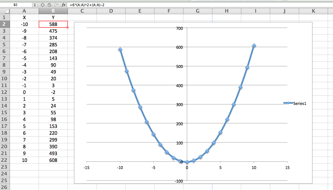
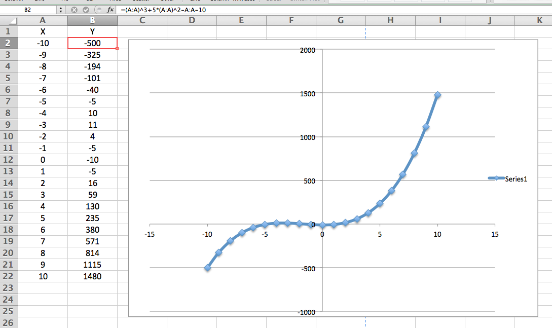
If this is confusing, I am going to go into a step by step process for designing my linear graph. The same process can be followed for the quadratic and cubic graphs. For all of my graphs I let the domain be the same (-10 ≤ x ≤ 10).
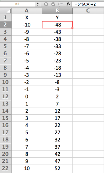
For my linear equation I set the equation to be y = 5x + 2. This can be inputted into the excel spreadsheet by clicking the column that is in the same row as the x value and typing
= 5*(A:A) + 2
The A:A is a shortcut so that the user does not have to do each X value for every individual row. A is the column that I decided to have my X values at while B is the column that I decided to have my Y values at.
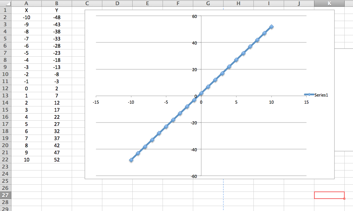
Then after that I clicked on Charts -> Scatter -> Smoth Marked Scatter to get the graph below.
Here is the equation I used for the quadratic function: y = 6x2 + x - 2. The same process can be used to create this graph.
Here is the equation I used for the cubic function: y = x3 + 5x2 - x - 10. The same process can be used to create this graph.
(All of these were constructed using the Microsoft Excel that was provided by the University of Georgia Aderhold Computer Labs)